G9 Tech Class #28

Today we will finish working on making the last touch ups to your Shares Tracker Product including:
It has to evidence the following specifications:

• use header rows
• sequence numbering
• sorting ascending and descending
• insert columns and rows
• column and row merge
• format title (font, color, size, shading, etc)
• at least three different formulas
• one fixed cell reference
• copy/cut and paste information
• insert a graph (pie, bar, etc)
• format the graph: change the Title: font & color, the colors of the bars/pie pieces, etc)

Record all your progress in your Process Journal before you turn in Create stage today (if you haven't turned it in last class).

Please make sure you are including the Assignment Standards and turn in your work by following the steps to submit and assignments.

G8 Tech Class #27

Today we do not have class due to the STAAR testing.
If you have not submitted Create stage, please do so before our next class on March 29.
Keep an eye on the Due Dates for Project 2 to stay on task.

Thanks.

G9 Tech Class #26

Today we will continue working on Create stage.

Please visit G9 Tech Class #25 for reviewing 

the expectations for Create stage.

Following the Due Dates for Project 2 Create stage is 
due today.

Please make sure you are including the 
Assignment Standards.

Before you submit Create stage today, don't forget to make your

 journal entry of the day and include in it the sketches of your designs

as visual evidence!

G9 Tech Class #25

Tech Class  #25!!! yahoo!

Today we will start working on Create stage. Please visit the G9 Due dates webpage to plan your time wisely.


You can look into Activity 8: from The NYSE Up Close and Personal Activity Booklet to review what are the expectations of the final product.

For this stage it is super important to look into these:

1. Your complete Process Journal with :

• dated journal entries including Visual Evidence (designs, sketches, screen shots, pictures, etc that show how the steps you took to create the product)
• notes regarding any changes made to Design and/or Plan: e.g. added a step, changed the order of tasks, changed the tools, used another resource, didn't need a resource, didn't finish what was planned etc.
• how did the group work? Did you have any issues? how did you overcome them, if any?

2. Explain what tools and techniques you used to create your product

3. How was your time management: Have you followed your time plan? How?

4. Have you made any changes to your chosen design? Why? How?

5. Complete your Shares tracking using all your spreadsheet knowledge following your chosen Design! :-) (Remember: you need to track your shares and record at least 6 changes in your shares)

You can always use the Design Folder Checklist to make sure your Create stage is complete.

Don't forget to make your journal entry of the day and  include in it all the screenshots of the process of creating your final product as visual evidence!

G9 Tech Class #24

Welcome back! Hope you all had a great Spring Break!

Continuing with Project 2, today we will work on Plan stage.

If you have not submitted Design stage and/or the Mix and Match (spreadsheet challenge) on March 8, you can turn them in today for 50% of the grade. For details on Design stage please visit:

G9 Tech Class #23

Remember that you can use the details for Mix and Match challenge listed on

G9 Tech Class #22 as your design specifications (what the final product needs to include to be successful! ;-)

In Plan stage you will be defining what will be done, when and with what resources. 

Focus on the process of creation of the final product to track your shares and "make" some money!

Remember to include:

• a step by step list of instructions to put together your spreadsheet to track your shares  (like giving very detailed instructions for someone else to build it for you!) 
• a detailed timeline (for the process of building/creation)
• the resources you will use
• Look at Due Dates for Project 2 and plan accordingly.
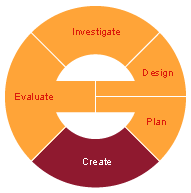
• For more info on Plan stage and tools to complete it, please revisit: G9 Tech Class #10

Today you will also need to start tracking your shares and follow their "behaviour".

Complete your Process Journal! Make your daily record of what you  learnt/progressed today.

G9 Tech Class #23

Today is our last class before Spring Break! :-)

Today is also International Women's day!

International Women's Day has been observed since in the early 1900's, a time of great expansion and turbulence in the industrialized world that saw booming population growth and the rise of radical ideologies.

1908
Great unrest and critical debate was occurring amongst women. Women's oppression and inequality was spurring women to become more vocal and active in campaigning for change. Then in 1908, 15,000 women marched through New York City demanding shorter hours, better pay and voting rights.

1909

In accordance with a declaration by the Socialist Party of America, the first National Woman's Day (NWD) was observed across the United States on 28 February. Women continued to celebrate NWD on the last Sunday of February until 1913.A global web of rich and diverse local activity connects women from all around the world ranging from political rallies, business conferences, government activities and networking events through to local women's craft markets, theatric performances, fashion parades and more.

Many global corporations have also started to more actively support IWD by running their own internal events and through supporting external ones. For example, on 8 March search engine and media giant Google some years even changes its logo on its global search pages. Year on year IWD is certainly increasing in status. The United States even designates the whole month of March as 'Women's History Month'.

So make a difference, think globally and act locally !! Make everyday International Women's Day. Do your bit to ensure that the future for girls is bright, equal, safe and rewarding.

Continue reading....

Please work on 4. Mix and Match explained in last class' blog post.

You also need to get in your groups and work on your Design stage for Project 2.

Please organize your group members' roles to start working on Design stage. 

Look into Activity 8: from The NYSE Up Close and Personal Activity Booklet to start your designs with the final product in mind...

Include a variety of different designs/proposed solutions  to show the information about your chosen stocks (at least 3)

Explain every part of each design

For explaining your designs, please use different techniques like story boards, sketches, labelled diagrams with explanations, etc.

Evaluate each design critically against the design specifications (assess what design specs each design meets or not)

Choose one design to build

Justify your choice of design that you will be using to track you shares

Look at Due Dates for Project 2 and plan accordingly.

G9 Tech Class #22

Today we will continue working with Spreadsheets:

Continuing last class' exercise 3. Sorting/Graphing/Percentages/Average: 

Part II:
Make your Percentage formula with a cell reference to the Max Grade cell using fixed cell reference (absolute range). Eg: 100


- Change the Max Grade in cell F2 to 200 and then change it again to 130 and see what happens to the results.
- Insert 2 columns between the columns named Grade and Percentage.
- Label those columns as Assignment/Test 2 and Grade 2.
- Complete these columns with assignments/test and grades information.

- Insert 1 column between the columns named Percentage and Max Grade.

- Label it: Average
- Under the Average column enter the formula to calculate the average between Grade and Grade 2.

- Insert three rows at the top
- Merge the rows and columns into one and add the title: "Students Grades for Spreadsheets class".

Part III:
- Select columns: Assignment/Test and Grade (including the header row)
- Insert a Bar Chart (What is this?)
- Place the graph/chart right under these columns Assignment/Test and Grade 
- Analyze the information graphed


- Repeat the same process using columns Assignment/Test 2 and Grade 2 (including the header row)
- select columns, insert bar chart, place graph under those columns, analyze the information graphed)




4. Mix and Match:
- Add a new Sheet and label it: 'My Challenge' 
- Create a challenge spreadsheet exercise including instructions, examples, etc for another group/student to solve. 
- It has to include the following design specifications:

1. use header rows
2. sequence numbering
3. sorting ascending and descending
4. insert columns and rows
5. column and row merge
6. format title (font, color, size, shading, etc)
7. three different formulas
8. one fixed cell reference
9. copy/cut and paste information
10. insert a graph (pie, bar, etc)
11. format the graph: change the Title: font & color, the colors of the bars/pie pieces, etc)

Type all the instructions and information on your "My Challenge" sheet. You can merge 5 columns by 5 rows for it.

G9 Tech Class #21

Today it's our first class in March!
Let's continue working on our spreadsheets!


2. Sorting 2: Go back to your sheet labelled 'Student List' and copy the set of data twice below leaving 2 black rows between each set. IN all, you will have 3 sets. Sort the groups by:
- alphabetically by Name
- alphabetically by last Name
- ascending by Age


Insert two rows at the top of each set of data. 
Merge the three columns and two rows into once cell. 

Type a title for each set of data explaining what the data is about. Eg: 
Student List sorted alphabetically (descending).
Change the font, formatting, etc any way you want (fonts, colors, shading, borders, etc...)

3. Sorting/Graphing/Percentages: In a new sheet labelled 'Teacher' create a set of data that shows the names of 15 actors/singers (as your students), the name of the assignment/test, and the grade they received (max=100). Add a column to number your students to the left. 
- Add a column/cell: Max Grade and type 100 under the title.
- Header row can be eg: Student # | Name | Assignment/Test |  Grade | Percentage | Max Grade

- Add a formula under the Percentage Title that shows what percentage of 100 each student received.


We will continue working on this exercise next class.